Tag Archives: R

Why I Switched to Julia

By: Bradley Setzler

Re-posted from: http://juliaeconomics.com/2014/06/15/why-i-started-a-blog-about-programming-julia-for-economics/

The following story, which I originally posted to The COBE Blog, explains why I began programming in Julia. Since then, I have found that Julia improves the performance of my other econometric estimators. However, Julia has a major disadvantage in that it lacks informative documentation and tutorials, much less accumulated discussion on sites like stackoverflow. This blog is meant to record the skills I am learning in Julia over time, to serve as a tutorial for economists and others learning the Julia programming language.


Is Julia the Future of Computational Economics?

Jorge Luis Garcia and I are currently estimating a structural econometric model of game-theoretic parent-child interaction. Using the standard implementation of Python (the code is written entirely in NumPy and SciPy with data prepared by Pandas), the optimizer ran for 24 hours, then terminated due to the 5,000 iteration limit. It was converging smoothly, but never quite arrived.

While waiting for the estimates last night (and growing increasingly impatient), I installed Julia and its packages, learned how to program in Julia, rewrote the estimation in Julia, and this morning successfully optimized the likelihood in Julia.

The contrast is staggering: the optimization that didn’t converge after 24 hours in Python converged after only 15 minutes in Julia while Python was still running on the same processor. Julia was already achieving a greater likelihood than Python after only 5 minutes even though Python had a 20-hour head start. They are both using the same optimization algorithm (including numerical tolerance), and the structure of the code is identical. Julia evaluates the likelihood in 0.5 seconds, while Python requires 21 seconds per evaluation, so Julia is about 40 times faster in the function evaluation, and about 100 times faster in the optimizer (I’m giving Python the benefit of the doubt even though it never converged).

The final iteration of Python was approaching the Julia optimal likelihood and getting closer; the only difference was that Julia arrived much, much more quickly. Since my next step is to bootstrap the estimator, speed is extremely important. Some practical arithmetic: on my four-core laptop, it would take two-thirds of a year to bootstrap this estimator 1,000 times, whereas Julia could do it in fewer than three days (though I’m planning to run the bootstrap in batch on the server).

I am agnostic on programming languages; I use whatever gets the answer fastest and can be reproduced most clearly, and I often use multiple languages on the same project to get the best features of each. My only claim is that Julia has taken the Python code, with minimal syntax changes, and executed the code 100 times faster for someone who had no prior experience with Julia. This was not a contrived, time-testing code; this is the estimator motivated by economic theory. The 100-fold speed increase of Julia relative to Python has been found elsewhere in computational economics.

So, is Julia the programming language of the future in structural econometrics? I’m not sure, but it seems to dominate Python and R at the moment.


Bradley J. Setzler


Prediction model for the FIFA World Cup 2014

By: Chris G

Re-posted from: https://grollchristian.wordpress.com/2014/06/12/world-cup-2014-prediction/

Like a last minute goal, so to speak, Andreas Groll and Gunther Schauberger of Ludwig-Maximilians-University Munich announced their predictions for the FIFA World Cup 2014 in Brazil – just hours before the opening game.

Andreas Groll, with his successful prediction of the European Championship 2012 already experienced in this field, and Gunther Schauberger did set out to predict the 2014 world cup champion based on statistical modeling techniques and R.

A bit surprisingly, Germany is estimated with highest probability of winning the trophy (28.80%), exceeding Brazil’s probability (the favorite according to most bookmakers) only marginally (27.65%). You can find all estimated probabilities compared to the respective odds from a German bookmaker in the graphic on their homepage (http://www.statistik.lmu.de/~schauberger/research.html), together with the most likely world cup evolution simulated from their model. The evolution also shows the neck-and-neck race between Germany and Brazil: they are predicted to meet each other in the semi-finals, where Germany’s probability of winning the game is a hair’s breadth above 50%. Although there does not exist a detailed technical report on the results yet, you still can get some insight into the model as well as the data used through a preliminary summary pdf on their homepage (http://www.statistik.lmu.de/~schauberger/WMGrollSchauberger.pdf).
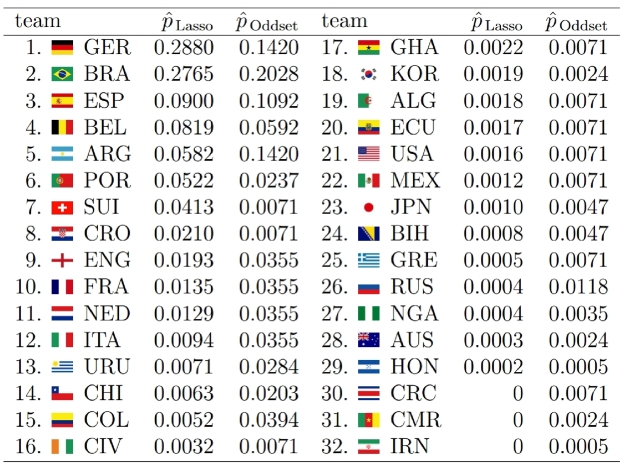
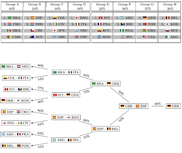
probs-001-001.jpg tree-001-001.jpg

Last week, I had the chance to witness a presentation of their preliminary results at the research seminar of the Department of Statistics (a home game for both), where they presented an already solid first predictive model based on the glmmLasso R package. However, continuously refining the model to the last minute, it now did receive its final touch, as they published the predictions at their homepage.

As they pointed out, statistical prediction of the world cup champion builds on two separate components. First, you need to reveal the individual team strengths – “who is best?”, so to speak. Afterwards, you need to simulate the evolution of the championship, given the actual world cup group drawings. This accounts for the fact that even quite capable teams might still miss the playoffs, given that they were drawn into a group of hard competitors.

Revealing the team strength turns out to be the hard part of the problem, as there exists no simple linear ranking for teams from best to worst. A team that might win more games on average still could have its problems with a less successful team, simply because they fail to adjust to the opponents style of play. In other words: tough tacklings and fouls could be the skillful players’ death.

Hence, Andreas Groll and Gunther Schauberger chose a quite complex approach: they determine the odds of a game through the number of goals that each team is going to score. Thereby, again, the likelihood of scoring more goals than the opponent depends on much more than just a single measure of team strength. First, the number of own goals depends on both teams’ capabilities: your own, as well as that of your opponent. As mediocre team, you score more goals against underdogs than against title aspirants. And second, your strength might be unevenly distributed across different parts of the team: your defense might be more competitive than your offensive or the other way round. As an example, although Switzerland’s overall strength is not within reach to the most capable teams, their defense during the last world cup still was such insurmountable that they did not receive a single goal (penalty shooting excluded).

The first preliminary model shown in the research seminar did seem to do a great job in revealing overall team strength already. However, subtleties as the differentiation between offensive and defense were not included yet. The final version, in contrast, now even allows such a distinction. Furthermore, the previous random effects model did build its prediction mainly on the data of past results itself, referring to explanatory co-variates only minor. Although this in no way indicates any prediction inaccuracies, one still would prefer models to have a more interpretable structure: not only knowing WHICH teams are best, but also WHY. Hence, instead of directly estimating team strength from past results, it is much nicer to have them estimated as a result of two components: the strength predicted by co-variates like FIFA rank, odds, etc, plus a small deviation found by the model through past results itself. As a side effect, the model should also become more robust against structural breaks this way: a team with very poor performance in the past now still could be classified as good if indicators of current team strength (like the number of champions league players or the current odds) hint to higher team strength.

Building on explanatory variables, however, the efficient identification of variables with true explanatory power out of a large set of possible variables is the real challenge. Hence, instead of throwing in all variables at once, their regularization approach allows to gradually extend the model by incorporating the variable with best explanatory power among all not yet included variables. This variable selection seems to me to be the big selling point of their statistical model, and with both Andreas Groll and Gunther Schauberger having prior publications in the field already, they most likely should know what they are doing.

From what I have heard, I think we can expect a technical report with more detailed analysis within the next weeks. I’m already quite excited about getting to know how large the estimated distinction between offensive and defense actually turns out to be in their model. Hopefully, we will get these results at a still early stage of the running world cup. The problem, however, is that some explanatory variables within their model could only be determined completely when all the team’s actual squads were known, and hence they could start their analysis only very shortly prior to the beginning of the world cup. Although this obviously caused some delay for their analysis, this made sure that even possible changes of team strength due to injuries could be taken into account. I am quite sure, however, that they will catch up on the delay during the next days, as I think that they are quite big football fans themselves, and hence are most likely as curious about the detailed results as we are…

Filed under: R Tagged: 2014 world cup, football, prediction, Rbloggers

Julia versus R – Playing around

By: Alvaro "Blag" Tejada Galindo

Re-posted from: http://blagrants.blogspot.com/2014/05/julia-versus-r-playing-around.html

So…as time goes by, I’m getting more proficient with Julia…which is something fairly easy as the learning curve is pretty fast…

I decided to load a file with 590,209 records that I got from Freebase…the file in question contains Actors and Actresses from movies…you can have a quick look here…

For this test, I’m using my Linux box on VMWare running on 2 GB of RAM…running Ubuntu 12.04.4 (Precise)

For R, I’m not using any special package…just plain R…version 2.14.1 and for Julia version 0.2.1, I’m using the DataFrames package…

Let’s take a look at the R source code first along with its runtime processing…

Actors_Info.R
start.time <- Sys.time()
if(!exists("Actors")){
Actors<-read.csv("Actors_Table.csv", header=TRUE, 
                     stringsAsFactors=FALSE, colClasses="character", na.strings = "")
}
Actors<-unique(Actors)
Actors<-Actors[complete.cases(Actors),]
Actor_Info<-data.frame(Actor_Id=Actors$Actor_Id,Name=Actors$Name,Gender=Actors$Gender)
Actor_Info<-Actor_Info[order(Actor_Info$Gender),]
write.csv(Actor_Info,"Actor_Info_R.csv",row.names=TRUE)
end.time <- Sys.time()
time.taken <- end.time - start.time
time.taken

This source will first ask if the file was loaded already, if not…it will load it…then, it will eliminate the repeated records, delete all the null or NA’s and the create a new Data Frame, sort it by “Gender” and then write a new CSV file…time will be taken to measure its speed…we will run it twice…first time the file is not loaded…second time it will…and that should improve greatly the execution time…

As we can see…the times are really good…and the different between the first and second run are pretty obvious…for the record…the generated file contains 105874 records…
Now…let’s see the Julia version of the code…
Actors_Info.jl
using DataFrames
start = time()
isdefined(:Actors) || (Actors = readtable("Actors_Table.csv", header=true, nastrings=["","NA"]))
drop_duplicates!(Actors)
complete_cases!(Actors)
Actor_Info = DataFrame(Actor_Id=Actors["Actor_Id"],Name=Actors["Name"],Gender=Actors["Gender"])
sortby!(Actor_Info, [:Gender])
writetable("Actor_Info_Julia.csv", Actor_Info)
finish = time()
println("Time: ", finish-start)


Here…we’re doing the same…we load the DataFrames package (But exclude that from the execution time), check if the file is loaded so we don’t load it again on the second run…eliminate duplicates, delete all null or NA, create a new DataFrame, sort it by “Gender” and finally write a new CVS file…

Well…the difference between the second and first run is very significative…but of course…way slower than R…
But…let me tell you one simple thing…Julia is still a brand new language…the DataFrames package is not part of the core Julia language, which means…that its even newer…and optimizations are being performed as we speak…I would say that for a young language…18 seconds to process 590,209 records is pretty awesome…and of course…my R experience surpasses greatly my Julia experience…

So…I don’t really want to leave you with the impression that Julia is not good or not fast enough…because believe me…it is…and you going to love my next experiment -;)

Let’s take a look at the R source code first…

Random_Names.R
start.time <- Sys.time()
names<-c("Anne","Gigi","Blag","Juergen","Marek","Ingo","Lars","Julia",
"Danielle","Rocky","Julien","Uwe","Myles","Mike", "Steven")

last_names<-c("Hardy","Read","Tejada","Schmerder","Kowalkiewicz","Sauerzapf",
"Karg","Satsuta","Keene","Ongkowidjojo","Vayssiere","Kylau",
"Fenlon","Flynn","Taylor")
full_names<-c()
for(i in 1:100000){
name<-sample(1:15, 1)
last_name<-sample(1:15, 1)
full_name<-paste(names[name],last_names[last_name],sep=" ")
full_names<-append(full_names,full_name)
}
end.time <- Sys.time()
time.taken <- end.time - start.time
time.taken

So this code is fairly simple…we have a couple of vectors with names and last names…then we loop 100000 times and then generate a couple of random numbers simply to read the vectors, create a full name and populate a new vector… with some random funny name combinations…

Well….the different between both runs is not really good…second time was a little bit higher…and 1 minute is kind of a lot…let’s see how Julia behaves…

Here’s the Julia source code…

Random_Numbers.jl
start = time()
names=["Anne","Gigi","Blag","Juergen","Marek","Ingo","Lars","Julia",
"Danielle","Rocky","Julien","Uwe","Myles","Mike", "Steven"]
last_names=["Hardy","Read","Tejada","Schmerder","Kowalkiewicz","Sauerzapf",
"Karg","Satsuta","Keene","Ongkowidjojo","Vayssiere","Kylau","Fenlon","Flynn","Taylor"]
full_names=String[]
full_name = ""
for i = 1:100000
name=rand(1:15)
last_name=rand(1:15)
full_name = names[name] * " " * last_names[last_name]
push!(full_names,full_name)
end
finish = time()
println("Time: ", finish-start)

So this code as well, creates two arrays with names and last names, do a loop 100000 times, generate a couple of random numbers, mix a name with a last name and then populate a new array with some mixed full names…

Just like in the R code…the second time took Julia a little bit more…but…less than a second?! That’s something like…amazingly fast and really took R by storm…
Now…I believe you will start to take Julia more seriously -:D
Hope you liked this blog…
Greetings,
Blag.
Development Culture.