After World Cup 2014 we finally are facing the next spectacular football event now: Euro 2016. With billions of football fans spread all over the world, football still seems to be the single most popular sport. Might have something to do with the fact that football is a game of underdogs: David could beat Goliath any day. Just take a look at the marvelous story of underdog Leicester City in this year’s Premier League season. It is this high uncertainty in future match outcomes that keeps everybody excited and puzzled about the one question: who is going to win?
A question, of course, that just feels like a perfectly designed challenge for data science, with an ever increasing wealth of football match statistics and other related data that is freely available nowadays. It comes as no surprise, hence, that Euro 2016 also puts statistics and data mining into the spotlight. Next to “who is going to win?”, the second question is: “who is going to make the best forecast?”
Besides the big players of the industry, whose predictions traditionally get the most of the media attention, there also is a less known academic research group that already had remarkable success in forecasting in the past. Andreas Groll and Gunther Schauberger from Ludwig-Maximilians-University, together with Thomas Kneib from Georg-August-University, again did set out to forecast the next Euro champion, after they already were able to predict the champion of Euro 2012 and World Cup 2014 correctly.
Based on publicly available data and the gamlls R-package they built a model to forecast probabilities of win, tie and loss for any game of Euro 2016 (Actually, they even get probabilities on a more precise level with an exact number of goals for both teams. For more details on the model take a look at their preliminary technical report).
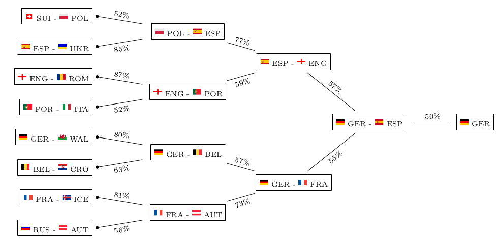
This is what their model deems as most likely tournament evolution this time:
The model not only takes into account individual team strengths, but also the group constellations that were randomly drawn and also have an influence on the tournament’s outcome. This is what their model predicts as probabilities for each team and each possible achievement in the tournament:
So good news for all Germans: after already winning World Cup 2014, “Die Mannschaft” seems to be getting its hands on the next big international football title!
Well, do they? Let’s see…
Mainstream media usually only picks up on the prediction of the Euro champion – the “point forecast”, so to speak. Keep in mind that although this single outcome may well be the most likely one, it still is quite unlikely itself with a probability of 21.1% only. So from a statistical point of view, you basically should not judge the model only on grounds of whether it is able to predict the champion again, as this would require a good portion of luck, too. Just imagine the probability of the most likely champion was 30%, then getting it correctly three times in a row merely has a probability of (0.3)³=0.027 or 2.7%. So in order to really evaluate the goodness of the model you need to check its forecasting power on a number of games and see whether it consistently does a good job, or even outperforms bookmakers’ odds. Although the report does not list the probabilities for each individual game, you still can get a quite good feeling about the goodness of the model, for example, by looking at the predicted group standings and playoff participants. Just compare them to what you would have guessed yourself – who’s the better football expert?
More often that I would like, I receive datasets where the data has only been partially cleaned, such as the picture on the right: hundreds, thousands…even millions of tiny files. Usually when this happens, the data all have the same format (such as having being generated by sensors or other memory-constrained devices).
The problem with data like this is that 1) it’s inconvenient to think about a dataset as a million individual pieces 2) the data in aggregate are too large to hold in RAM but 3) the data are small enough where using Hadoop or even a relational database seems like overkill.
Surprisingly, with judicious use of GNU Parallel, stream processing and a relatively modern computer, you can efficiently process annoying, “medium-sized” data as described above.
The cat utility in Unix-y systems is familiar to most anyone who has ever opened up a Terminal window. Take some or all of the files in a folder, concatenate them together….one big file. But something funny happens once you get enough files…
$ cat * >> out.txt
-bash: /bin/cat: Argument list too long
That’s a fun thought…too many files for the computer to keep track of. As it turns out, many Unix tools will only accept about 10,000 arguments; the use of the asterisk in the cat command gets expanded before running, so the above statement passes 1,234,567 arguments to cat and you get an error message.
One (naive) solution would be to loop over every file (a completely serial operation):
for f in *; do cat "$f" >> ../transactions_cat/transactions.csv; done
Roughly 10,093 seconds later, you’ll have your concatenated file. Three hours is quite a coffee break…
Solution 1: GNU Parallel & Concatenation
Above, I mentioned that looping over each file gets you past the error condition of too many arguments, but it is a serial operation. If you look at your computer usage during that operation, you’ll likely see that only a fraction of a core of your computer’s CPU is being utilized. We can greatly improve that through the use of GNU Parallel:
ls | parallel -m -j $f "cat {} >> ../transactions_cat/transactions.csv"
The $f argument in the code is to highlight that you can choose the level of parallelism; however, you will not get infinitely linear scaling, as shown below (graph code, Julia):
Given that the graph represents a single run at each level of parallelism, it’s a bit difficult to say exactly where the parallelism gets maxed out, but at roughly 10 concurrent jobs, there’s no additional benefit. It’s also interesting to point out what the −m argument represents; by specifying m, you allow multiple arguments (i.e. multiple text files) to be passed as inputs into parallel. This alone leads to an 8x speedup over the naive loop solution.
Problem 2: Data > RAM
Now that we have a single file, we’ve removed the “one million files” cognitive dissonance, but now we have a second problem: at 19.93GB, the amount of data exceeds the RAM in my laptop (2014 MBP, 16GB of RAM). So in order to do analysis, either a bigger machine is needed or processing has to be done in a streaming or “chunked” manner (such as using the “chunksize” keyword in pandas).
But continuing on with our use of GNU Parallel, suppose we wanted to answer the following types of questions about our transactions data:
How many unique products were sold?
How many transactions were there per day?
How many total items were sold per store, per month?
If it’s not clear from the list above, in all three questions there is an “embarrassingly parallel” portion of the computation. Let’s take a look at how to answer all three of these questions in a time- and RAM-efficient manner:
Q1: Unique Products
Given the format of the data file (transactions in a single column array), this question is the hardest to parallelize, but using a neat trick with the `tr` (transliterate) utility, we can map our data to one product per row as we stream over the file:
This file contains bidirectional Unicode text that may be interpreted or compiled differently than what appears below. To review, open the file in an editor that reveals hidden Unicode characters.
Learn more about bidirectional Unicode characters
The trick here is that we swap the comma-delimited transactions with the newline character; the effect of this is taking a single transaction row and returning multiple rows, one for each product. Then we pass that down the line, eventually using sort−u to de-dup the list and wc−l to count the number of unique lines (i.e. products).
In a serial fashion, it takes quite some time to calculate the number of unique products. Incorporating GNU Parallel, just using the defaults, gives nearly a 4x speedup!
Q2. Transactions By Day
If the file format could be considered undesirable in question 1, for question 2 the format is perfect. Since each row represents a transaction, all we need to do is perform the equivalent of a SQL GroupBy on the date and sum the rows:
This file contains bidirectional Unicode text that may be interpreted or compiled differently than what appears below. To review, open the file in an editor that reveals hidden Unicode characters.
Learn more about bidirectional Unicode characters
Using GNU Parallel starts to become complicated here, but you do get a 9x speed-up by calculating rows by date in chunks, then “reducing” again by calculating total rows by date (a trick I picked up at this blog post).
Q3. Total items Per store, Per month
For this example, it could be that my command-line fu is weak, but the serial method actually turns out to be the fastest. Of course, at a 14 minute run time, the real-time benefits to parallelization aren’t that great.
This file contains bidirectional Unicode text that may be interpreted or compiled differently than what appears below. To review, open the file in an editor that reveals hidden Unicode characters.
Learn more about bidirectional Unicode characters
# Serial method uses 40-50% all available CPU prior to sort step. Assuming linear scaling, best we could achieve is halving the time.
# Grand Assertion: this pipeline actually gives correct answer! This is a very complex way to calculate this, SQL would be so much easier...
# cut -d ' ' -f 2,3,5 - Take fields 2, 3, and 5 (store, timestamp, transaction)
# tr -d '[A-Za-z\"/\- ]' - Strip out all the characters and spaces, to just leave the store number, timestamp, and commas to represent the number of items
# awk '{print (substr($1,1,5)"-"substr($1,6,6)), length(substr($1,14))+1}' - Split the string at the store, yearmo boundary, then count number of commas + 1 (since 3 commas = 4 items)
# awk '{a[$1]+=$2;}END{for(i in a)print i" "a[i];}' - Sum by store-yearmo combo
# sort - Sort such that the store number is together, then the month
It may be possible that one of you out there knows how to do this correctly, but an interesting thing to note is that the serial version already uses 40-50% of the available CPU available. So parallelization might yield a 2x speedup, but seven minutes extra per run isn’t worth spending hours trying to the optimal settings.
But, I’ve got MULTIPLE files…
The three examples above showed that it’s possible to process datasets larger than RAM in a realistic amount of time using GNU Parallel. However, the examples also showed that working with Unix utilities can become complicated rather quickly. Shell scripts can help move beyond the “one-liner” syndrome, when the pipeline gets so long you lose track of the logic, but eventually problems are more easily solved using other tools.
The data that I generated at the beginning of this post represented two concepts: transactions and customers. Once you get to the point where you want to do joins, summarize by multiple columns, estimate models, etc., loading data into a database or an analytics environment like R or Python makes sense. But hopefully this post has shown that a laptop is capable of analyzing WAY more data than most people believe, using many tools written decades ago.
Julia has native support for calling C and FORTRAN functions. There are also add on packages which provide interfaces to C++, R and Python. We’ll have a brief look at the support for C and R here. Further details on these and the other supported languages can be found on github.
Why would you want to call other languages from within Julia? Here are a couple of reasons:
to access functionality which is not implemented in Julia;
to exploit some efficiency associated with another language.
The second reason should apply relatively seldom because, as we saw some time ago, Julia provides performance which rivals native C or FORTRAN code.
C
C functions are called via ccall(), where the name of the C function and the library it lives in are passed as a tuple in the first argument, followed by the return type of the function and the types of the function arguments, and finally the arguments themselves. It’s a bit klunky, but it works!
This function will not be vectorised by default (just try call csqrt() on a vector!), but it’s a simple matter to produce a vectorised version using the @vectorize_1arg macro.
julia> @vectorize_1arg Real csqrt;
julia> methods(csqrt)
# 4 methods for generic function "csqrt":
csqrt{T<:Real}(::AbstractArray{T<:Real,1}) at operators.jl:359
csqrt{T<:Real}(::AbstractArray{T<:Real,2}) at operators.jl:360
csqrt{T<:Real}(::AbstractArray{T<:Real,N}) at operators.jl:362
csqrt(x) at none:6
Note that a few extra specialised methods have been introduced and now calling csqrt() on a vector works perfectly.
I’ll freely admit that I don’t dabble in C too often these days. R, on the other hand, is a daily workhorse. So being able to import R functionality into Julia is very appealing. The first thing that we need to do is load up a few packages, the most important of which is RCall. There’s great documentation for the package here.
julia> using RCall
julia> using DataArrays, DataFrames
We immediately have access to R’s builtin data sets and we can display them using rprint().
julia> rprint(:HairEyeColor)
, , Sex = Male

       Eye
Hair    Brown Blue Hazel Green
  Black    32   11    10     3
  Brown    53   50    25    15
  Red      10   10     7     7
  Blond     3   30     5     8

, , Sex = Female

       Eye
Hair    Brown Blue Hazel Green
  Black    36    9     5     2
  Brown    66   34    29    14
  Red      16    7     7     7
  Blond     4   64     5     8
We can also copy those data across from R to Julia.
However, for some complex objects there is no simple way to translate between R and Julia, and in these cases rcopy() fails. We can see in the case below that the object of class lm returned by lm() does not diffuse intact across the R-Julia membrane.
julia> "fit <- lm(bwt ~ ., data = MASS::birthwt)" |> rcopy
ERROR: `rcopy` has no method matching rcopy(::LangSxp)
 in rcopy at no file
 in map_to! at abstractarray.jl:1311
 in map_to! at abstractarray.jl:1320
 in map at abstractarray.jl:1331
 in rcopy at /home/colliera/.julia/v0.3/RCall/src/sexp.jl:131
 in rcopy at /home/colliera/.julia/v0.3/RCall/src/iface.jl:35
 in |> at operators.jl:178
But the call to lm() was successful and we can still look at the results.
You can use R to generate plots with either the base functionality or that provided by libraries like ggplot2 or lattice.
julia> reval("plot(1:10)");                # Will pop up a graphics window...
julia> reval("library(ggplot2)");
julia> rprint("ggplot(MASS::birthwt, aes(x = age, y = bwt)) + geom_point() + theme_classic()")
julia> reval("dev.off()")                  # ... and close the window.
Watch the videos below for some other perspectives on multi-language programming with Julia. Also check out the complete code for today (including examples with C++, FORTRAN and Python) on github.


 by
by