Given a polynomial of degree with values

defined for a window of size ,

We want to find the value of its k-order derivative in the middle of the window assuming that the are founded solving a least-squares problem:

where is our signal values and is the Vandermonde matrix:

using the normal equation

and a QR decomposition, we get

now we can express all the polynomial values in a vector . Lets rewrite this in matrix form:

Now the “big trick” is to write the Taylor series and to remember that this formula is exact for polynomial functions:

Lets rewrite this in matrix form:

With a good eye we see that where is a diagonal matrix:

That’s all, we only have to group pieces:

With the QR decomposition and we get:

using the fact that we get:

hence we have:

which is our final formula.

We can use mathematica to do a symbolic computation using .

For a window width of points and a polynomial of degree we get:

n = 3; d = 2;
V = Table[If[j != 0, i^j, 1], {i, -n, n}, {j, 0, d}];
{Qt, R} = QRDecomposition[V];
DD = DiagonalMatrix[Table[Factorial[i], {i, 0, d}]];
DD.Inverse[R].Qt // TeXForm

The first row is the smoothing filter, the second one the smoothed first order derivative filter and the last one the smoothed second order derivative filter.

Here I present a direct implementation in julia.

We first initialize a Vandermonde matrix:

function vandermonde(halfWindow::Int, polyDeg::Int,T::Type=Float64)
    
    @assert halfWindow>=0
    @assert polyDeg>=0
    
    x=T[i for i in -halfWindow:halfWindow]

    n = polyDeg+1
    m = length(x)
    
    V = Array{T}(m, n)
    
    for i = 1:m
        V[i,1] = T(1)
    end
    for j = 2:n
        for i = 1:m
            V[i,j] = x[i] * V[i,j-1]
        end
    end

    return V
end

We then compute the filter coefficients with the presented formula.

Attention we return the transposed matrix because in Julia it is more convenient to use SG[:,1] which is a julia vector. SG[1,:] would be a (1,n) julia matrix.

function SG(halfWindow::Int, polyDeg::Int,T::Type=Float64)

    @assert 2*halfWindow>polyDeg
    
    V=vandermonde(halfWindow,polyDeg,T)
    Q,R=qr(V)
    SG=R\Q'

    for i in 1:size(SG,1)
        SG[i,:]*=factorial(i-1)
    end
    
# CAVEAT: returns the transposed matrix

    return SG'
end

The final step to use the filter is to provide function to do the cross-correlation.

I do not want to talk too much about this subroutine because in a future post I will show how to efficiently compute such kind of convolution. Here we use a FFT, but with a short filter it is much more efficient (around 10 times faster) to use a direct computation. I will show how to implement

which can be used to compute discrete and stationary wavelet transform for instance.

One last thing, here we use constant padding to manage the boundaries.

function apply_filter{T}(filter::StridedVector{T},signal::StridedVector{T})

    @assert isodd(length(filter))

    halfWindow = round(Int,(length(filter)-1)/2)
    
    padded_signal = 
        [signal[1]*ones(halfWindow);
         signal;
         signal[end]*ones(halfWindow)]

    filter_cross_signal = conv(filter[end:-1:1], padded_signal)

    return filter_cross_signal[2*halfWindow+1:end-2*halfWindow]
end

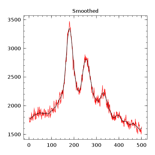
Finally I have included a small usage example. To see well the effect of Savitzky-Golay filters, I have over smoothed with a large window width ,

using Winston

s=readdlm("signal.txt")[:,1]

sg=SG(20,3) # halt-window, polynomal degree

#________________

smoothed=apply_filter(sg[:,1],s)

plot(s,"r")
oplot(smoothed)
title("Smoothed")
savefig("smoothed.png")

#________________

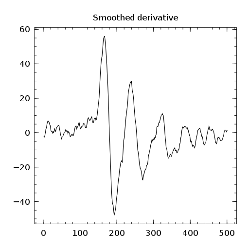
smoothed_d1=apply_filter(sg[:,2],s)

plot(smoothed_d1)
title("Smoothed derivative")
savefig("smoothed_d1.png")

#________________

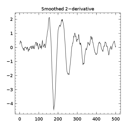
smoothed_d2=apply_filter(sg[:,3],s)

plot(smoothed_d2)
title("Smoothed 2-derivative")
savefig("smoothed_d2.png")

Here is the resulting plots:

To reproduce these figures you can find the complete code on github.