Re-posted from: http://www.stochasticlifestyle.com/multiple-gpu-on-the-hpc-with-julia/
This is the exciting Part 3 to using Julia on an HPC. First I got you started with using Julia on multiple nodes. Second, I showed you how to get the code running on the GPU. That gets you pretty far. However, if you got a trial allocation on Cometand started running jobs, you may have noticed when looking at the architecture that you’re not getting to use the full GPU. In the job script I showed you, I asked for 2 GPUs. Why? Well, that’s because the flagship NVIDIA GPU, the Tesla K80, is actually a duel GPU and you have to control the two parts separately. You may have been following along on your own computer and have been wondering how you use the multiple GPUs in your setup as well. This tutorial will cover how to extend our function to multiple-GPU setups. You will notice that while this code was made for 2 GPUs, by simply extended the array  with the values of other GPUs then this code automatically extends to however many you need.
Recall
I want to recall the problem a bit to rephrase it and make it easier to understand why what we are doing will work. Recall that we are simply looping over a mesh of  (you can think of it as
  ) and solving some inner function at each point, and add together the results. The CUDA kernal is shown in the previous part. Thus, how we will extend our problem to multiple GPUs is to simply split the mesh and solve the inner function on different GPUs. It’s critical to realize that this solution method requires independence, i.e. that different parts of the grid do not effect each other. Thus you can think of our function as being a “vectorized” evaluation.
Note that we are not doing the most memory efficient implementation. Each GPU will have the full array of  ‘s and
  ‘s even though they will only evaluate it at specific parts. One could split it up, though that would take more work for little performance gain. Thus you should really look into this if you are running low on memory (or to do as an exercise). If you would like to do this, then you can calculate how far in the ‘s the first GPU calculates, and then only send the right portion of the ‘s to the other GPU (since we loop down the ‘s, both will need the full array). Since this problem is not memory limited, I will not show this solution.
Upgrading the Kernal
Upgrading the kernal will be quite simple. Recall that we had the problem in linear indexing before. We will keep the linear indexing, except in each GPU we will pass an integer, StartIdx, which will tell the GPU where in the linear indexing it will start. Thus as before we had the value  which told the GPU how many indices each core will evaluate, and we had
int index = threadIdx.x + blockIdx.x * blockDim.x;
which tells the GPU which core it is, we have a new global index which is
int globalIndex = index*equalDiv+startIdx;
Notice that each  is apart, and so that is the section each GPU will operate on. The CUDA kernal then just sums up the solution of the inner function over the next indices:
    __global__ void integration(const float *coefs, const float *iArr, const float *jArr, const int sizei, const int sizej, const int equalDiv,const int startIdx, int *tmp)
    {
        int index = threadIdx.x + blockIdx.x * blockDim.x;
        int globalIndex = index*equalDiv+startIdx;
        int loopInd;
        float i;
        float j;
        float isq2;
        float isq3;
        float isq4;
        float isq5;
        float isq6;
        float isq7;
        float isq8;
        float jsq2;
        float jsq3;
        float jsq4;
        float jsq5;
        float jsq6;
        float jsq7;
        float jsq8;
        int ans = 0;
        for(loopInd=0;loopInd<equalDiv;loopInd=loopInd+1){
          i = iArr[(globalIndex+loopInd)/sizej];
          j = jArr[(globalIndex+loopInd)%sizej];
          if(globalIndex+loopInd >= sizei*sizej){
            break;
          }
          if((globalIndex+loopInd)%sizej==0 || loopInd==0){
            isq2 = i*i;
            isq3 = i*isq2;
            isq4 = isq2*isq2;
            isq5 = i*isq4;
            isq6 = isq4*isq2;
            isq7 = i*isq6;
            isq8 = isq4*isq4;
          }
          jsq2 = j*j;
          jsq3 = j*jsq2;
          jsq4 = jsq2*jsq2;
          jsq5 = j*jsq4;
          jsq6 = jsq2*jsq4;
          jsq7 = j*jsq6;
          jsq8 = jsq4*jsq4;
          ans = ans + innerFunc(coefs,i,isq2,isq3,isq4,isq5,isq6,isq7,isq8,j,jsq2,jsq3,jsq4,jsq5,jsq6,jsq7,jsq8);
        }
        tmp[index] = ans;
    }
Notice that the inner function did not have to be changed at all:
  __device__ int innerFunc(const float *coefs,const float i,const float isq2,const float isq3,const float isq4,const float isq5,const float isq6,const float isq7,const float isq8,const float j,const float jsq2,const float jsq3,const float jsq4,const float jsq5,const float jsq6,const float jsq7,const float jsq8)
  {
    return abs(coefs[0]*(jsq2) + coefs[1]*(jsq3) + coefs[2]*(jsq4) + coefs[3]*(jsq5) + coefs[4]*jsq6 + coefs[5]*jsq7 + coefs[6]*jsq8 + coefs[7]*(i) + coefs[8]*(i)*(jsq2) + coefs[9]*i*jsq3 + coefs[10]*(i)*(jsq4) + coefs[11]*i*jsq5 + coefs[12]*(i)*(jsq6) + coefs[13]*i*jsq7 + coefs[14]*(isq2) + coefs[15]*(isq2)*(jsq2) + coefs[16]*isq2*jsq3 + coefs[17]*(isq2)*(jsq4) + coefs[18]*isq2*jsq5 + coefs[19]*(isq2)*(jsq6) + coefs[20]*(isq3) + coefs[21]*(isq3)*(jsq2) + coefs[22]*isq3*jsq3 + coefs[23]*(isq3)*(jsq4) + coefs[24]*isq3*jsq5 + coefs[25]*(isq4) + coefs[26]*(isq4)*(jsq2) + coefs[27]*isq4*jsq3 + coefs[28]*(isq4)*(jsq4) + coefs[29]*(isq5) + coefs[30]*(isq5)*(jsq2) + coefs[31]*isq5*jsq3+ coefs[32]*(isq6) + coefs[33]*(isq6)*(jsq2) + coefs[34]*(isq7) + coefs[35]*(isq8))<1;
  }
As before, we wrap this in extern “C”{} for libraries.
Setup Multi-GPU Julia Driver
Recall that we are starting with the following parameters:
  imin = -12
  imax = 1
  jmin = -4
  jmax = 4
  iarr = convert(Vector{Float32},collect(imin:dx:imax))
  jarr = convert(Vector{Float32},collect(jmin:dx:jmax))
  sizei = length(imin:dx:imax)
  sizej = length(jmin:dx:jmax)
  totArea = ((imax-imin)*(jmax-jmin)/(sizei*sizej));

  coefs = getCoefficients(A0,A1,B0,B1,α,β1,β2,β3,β4)
Where getCoefficients is some function which returns an array of 36 integers. You can make this be a call for random integers or something of the like. Now we need to call our kernal from Julia. Start by compling the kernal as in part two into a .ptx. Our simple implementation will be to split the job by the number of cores on each GPU. On Comet, each part of the K80 has 2496 CUDA cores, so we would set
cudaCores = [2496,2496]
I will instead use the more interesting case of my development computer. It has a GTX 970 with 1664 cores and a GTX 750Ti with 640 cores. Therefore I start by setting
cudaCores = [1664,640]
The implementation is then as follows: I first get as the number of calculations to be done per core. Since I am looping over a mesh with  and
and  , if I let
  be the total number of cores, then
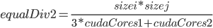
equalDiv = sizei*sizej÷totCores + 1
tells me how many calculations per core (we add 1 (or take the ceiling) in order to make sure that we cover all of it. Otherwise the part truncated from the integer division will not be calculated). Next we need to calculate where to start the second GPU. Let  be the total number of calculations in each GPU (it returns a vector of 2 values). I want my code to work when there’s only 1 card (i.e.
 ![cudaCores=[2946]](https://i2.wp.com/www.stochasticlifestyle.com/wp-content/plugins/latex/cache/tex_77145979839f0aa461fb95033ff1f5a4.gif) ), so to calculate the starting indices I run
), so to calculate the starting indices I run
  if numCards > 1
    startIdx = [0 cumsum(portions)[1:end-1]]
  else
    startIdx = [0]
  end
What this does is give an array where the first value is zero, the second value is portions[1], the third is portions[1]+portions[2], etc., and if there is only one card then it’s simply the array with zero. Notice this is exactly the index which the CUDA kernal needs to stop at, so this works.
Now we need to move our arrays over to the GPU. Note that each array is stored on only one GPU, and so we need to loop through the devices and put each array on each device. We change devices with with command device(i), where i=0 is the first device, i=1 is the second, etc. Since the values are actually C-pointers, we will just store them in arrays of type Any (of size  which is the number of GPU cards as calculated by the length(cudaCores)). The setup is then:
  g_iarr = Vector{Any}(numCards)
  g_jarr = Vector{Any}(numCards)
  g_tmp = Vector{Any}(numCards)
  g_coefs = Vector{Any}(numCards)
  ans = Vector{Int32}(numCards)
  integrationFuncs = Vector{Any}(numCards)
  CUDArt.init(devices(dev->true))
  devlist = devices(dev->true)
  streams = [(device(dev); Stream()) for dev in devlist]
  for i = 1:numCards
    device(i-1)
    g_iarr[i]  = CudaArray(iarr)
    g_jarr[i]  = CudaArray(jarr)
    g_tmp[i]   = CudaArray(Int32,cudaCores[i])
    md = CuModule("integration.ptx",false)
    integrationFuncs[i] = CuFunction(md,"integration")
  end
Lastly, we need to call the kernal. Recall that in my problem the inner loop is to change coefs, run the kernal calculation, and use the result. Thus in my test function is where I send coefs to the GPU. This will call the kernal as before, except we need to do this asynchronously via Julia’s streams. Notice we have a new variable (or array of variables) around: streams. The code initiated 2 GPU streams, one on each device. Thus what we will do is tell the kernal to run on the stream, and move onto the calculation before it finishes (but tell it to not sum the result until after the GPU stream finished). This is done by the following code:
        @async begin
          dev = device(i-1)
          g_coefs[i] = CudaArray(coefs)
          launch(integrationFuncs[i], cudaCores[i], 64, (g_coefs[i], g_iarr[i], g_jarr[i], sizei,sizej,equalDiv,startIdx[i],g_tmp[i],),stream=streams[i]);
          wait(streams[i])
          ans[i] = sum(to_host(g_tmp[i]))
        end
@async is the command which asynchronizes, as in Julia keeps going forward even if the command isn’t done. Thus what we need to do is run all of the GPUs and then wait for each to finish via the @sync command. The full loop is then as follows:
  function f4()
    @sync begin
      for i = 1:numCards
        @async begin
          dev = device(i-1)
          g_coefs[i] = CudaArray(coefs)
          launch(integrationFuncs[i], cudaCores[i], 64, (g_coefs[i], g_iarr[i], g_jarr[i], sizei,sizej,equalDiv,startIdx[i],g_tmp[i],),stream=streams[i]);
          wait(streams[i])
          ans[i] = sum(to_host(g_tmp[i]))
        end
      end
    end
    res = sum(ans)*totArea
    #println(res)
  end
I put it in the function f4 for benchmarking. Notice we have @sync around the inner loop, telling it not to go past the loop until each portion is done, but in the loop we wrap it with @async so that way Julia can start the GPU codes all at the same time without having to wait for the first to finish, and then as they finish it comes back to finish up (this is not needed to be done in parallel since the overhead for doing this is really small. The overhead of @parallel would probably increase the runtime!). After we are done, we scale the area to get the answer.
So how well did it do? On my last post someone told me to checkout the benchmark package. So to finish off the code I run:
  df4 = benchmark(f4,"MultiGPU",1000)
  println(df4)
  CUDArt.close(devices(dev->true))
benchmark will run the function 1000 times and tell me the average runtime by printing the dataframe df4. Then I close the GPU to clean up the memory.
Heterogeneous GPU Setup
Recall that our last implementation simply split up the problem by how many cores each GPU has. We will get back to whether that is correct or not later, but first lets make something a little more complicated to test this out. So what about making equalDiv higher on faster GPUs and slower on slower GPUs? What we will do is declare an array trueBias, like
trueBias = [.75,.25]
which will say how to bias the equalDivs amongst the GPUs. How do we calculate the division? It’s easiest to do this by example. Notice in the code above we have that

that is equalDiv is 3 times the size on the first GPU than the second GPU. Since the number of values we want to calculate is  , and we calculate values on
 ![cudaCores[i]](https://i2.wp.com/www.stochasticlifestyle.com/wp-content/plugins/latex/cache/tex_fcdf951de22da0e6201f3ff421a4614d.gif) different cores, the total amount that we calculate is
different cores, the total amount that we calculate is

and by substitution we then get
Do a bigger example with [.75, 1/16, 1/8, 1/16]. See the pattern? Notice that trueBias/trueBias[i] gives us the value that we need to substitute $k$ with $i$ (where $k$ is the value on the top). Then notice that the left hand side is simply the dot product of these values with the number of cudaCores. Thus we pull out  and sizei*sizej by that dot product to get what should be the final result is that the following calculates the desired quantity:
  equalDiv = Vector{Int32}(numCards)
  for i = 1:numCards
    equalDiv[i] = ceil(Int32,(sizei*sizej)/dot(trueBias/(trueBias[i]),cudaCores))
  end
We then need to make sure we scale portions by the equalDiv per GPU:
  portions = equalDiv.*cudaCores
  if numCards > 1
    startIdx = [0 cumsum(portions)[1:end-1]]
  else
    startIdx = [0]
  end
When calling the kernal, all we have to do is specify which equalDiv we want to use, and thus we get the test function:
  function f5()
    @sync begin
      for i = 1:numCards
        @async begin
          dev = device(i-1)
          g_coefs[i] = CudaArray(coefs)
          launch(integrationFuncs[i], cudaCores[i], 64, (g_coefs[i], g_iarr[i], g_jarr[i], sizei,sizej,equalDiv[i],startIdx[i],g_tmp[i],),stream=streams[i]);
          wait(streams[i])
          ans[i] = sum(to_host(g_tmp[i]))
        end
      end
    end
    res = sum(ans)*totArea
    #println(res)
  end
  df5 = benchmark(f5,"MultiGPU2",1000)
  println(df5)
  CUDArt.close(devices(dev->true))
Same as before with equalDiv[i] now.
Does Changing the Divisions Help?
I ran this on my desktop and got the following results:
1x12 DataFrames.DataFrame
| Row | Category | Benchmark | Iterations | TotalWall | AverageWall |
|-----|----------|-----------|------------|-----------|-------------|
| 1   | "GPU"    | "GPU"     | 1000       | 23.1013   | 0.0231013   |

| Row | MaxWall   | MinWall  | Timestamp             |
|-----|-----------|----------|-----------------------|
| 1   | 0.0264843 | 0.021724 | "2016-02-27 17:16:32" |

| Row | JuliaHash                                  | CodeHash | OS        |
|-----|--------------------------------------------|----------|-----------|
| 1   | "a2f713dea5ac6320d8dcf2835ac4a37ea751af05" | NA       | "Windows" |

| Row | CPUCores |
|-----|----------|
| 1   | 8        |
1x12 DataFrames.DataFrame
| Row | Category   | Benchmark  | Iterations | TotalWall | AverageWall |
|-----|------------|------------|------------|-----------|-------------|
| 1   | "MultiGPU" | "MultiGPU" | 1000       | 22.3445   | 0.0223445   |

| Row | MaxWall   | MinWall   | Timestamp             |
|-----|-----------|-----------|-----------------------|
| 1   | 0.0593403 | 0.0211532 | "2016-02-27 17:16:55" |

| Row | JuliaHash                                  | CodeHash | OS        |
|-----|--------------------------------------------|----------|-----------|
| 1   | "a2f713dea5ac6320d8dcf2835ac4a37ea751af05" | NA       | "Windows" |

| Row | CPUCores |
|-----|----------|
| 1   | 8        |
1x12 DataFrames.DataFrame
| Row | Category    | Benchmark   | Iterations | TotalWall | AverageWall |
|-----|-------------|-------------|------------|-----------|-------------|
| 1   | "MultiGPU2" | "MultiGPU2" | 1000       | 22.5787   | 0.0225787   |

| Row | MaxWall   | MinWall   | Timestamp             |
|-----|-----------|-----------|-----------------------|
| 1   | 0.0557531 | 0.0213999 | "2016-02-27 17:17:18" |

| Row | JuliaHash                                  | CodeHash | OS        |
|-----|--------------------------------------------|----------|-----------|
| 1   | "a2f713dea5ac6320d8dcf2835ac4a37ea751af05" | NA       | "Windows" |

| Row | CPUCores |
|-----|----------|
| 1   | 8        |
1x12 DataFrames.DataFrame
| Row | Category             | Benchmark            | Iterations | TotalWall |
|-----|----------------------|----------------------|------------|-----------|
| 1   | "MultiGPU2-Balanced" | "MultiGPU2-Balanced" | 1000       | 22.3453   |

| Row | AverageWall | MaxWall   | MinWall   | Timestamp             |
|-----|-------------|-----------|-----------|-----------------------|
| 1   | 0.0223453   | 0.0593927 | 0.0211599 | "2016-02-27 17:17:41" |

| Row | JuliaHash                                  | CodeHash | OS        |
|-----|--------------------------------------------|----------|-----------|
| 1   | "a2f713dea5ac6320d8dcf2835ac4a37ea751af05" | NA       | "Windows" |

| Row | CPUCores |
|-----|----------|
| 1   | 8        |
The first run was 1 GPU which averaged .0231 seconds. The second run was equal splitting which got .0223 seconds. Next was the split trueBias = [.51,.49] which got .0225 seconds. Lastly I set trueBias = [.5,.5] and got .0223 seconds. Thus notice two things: one allowing for the homogeneous split has no overhead (we still only pass an integer), but more interesting, the best split was still 50-50. This is reproducible and only gets worse when we split more ([.75,.25] is terrible!).
So what’s going on? Well, first of all notice that this is not a memory bound problem: in the loop we only send an array of 36 values. The largest difference between the GPUs is their memory bandwidth. From the GTX 970 specs we see that its memory bandwidth is 224 GB/sec, vs the GTX 750Ti’s 86.4 GB/sec. That’s a whopping 2.5x difference, but it doesn’t matter in this case. All that matters in this test is the compute power. Here the GTX 970 has a base clock of 1050 MHz and a boost clock of 1178 MHz, while the GTX 750Ti has a base clock of 1020 MHz and a boost clock of 1085 MHz. 1178/1085 = 1.08. They are almost the same. Note that this is the difference between a entry level graphics card from ~4 years ago, vs one of the high-end cards of today (only beat in the gaming sphere by the GTX 980(Ti) and the Titan X). GPUs tend to have about the same strength per core, while the difference is mostly in how many cores there are. In that sense, our result is not surprising. However, knowing how to deal with the heterogeneity is probably good for more memory taxing problems.
Running it on Comet
I compiled this code onto Comet and ran it with the job script
#!/bin/bash
#SBATCH -A uci128
#SBATCH --job-name="jOpt"
#SBATCH --output="output/jOpt.%j.%N.out"
#SBATCH --partition=gpu-shared
#SBATCH --gres=gpu:2
#SBATCH --nodes=1
#SBATCH --export=ALL
#SBATCH --mail-type=ALL
#SBATCH --mail-user=crackauc@uci.edu
#SBATCH --ntasks-per-node=12
#SBATCH -t 0:10:00
module load cuda/7.0
module load cmake
export SLURM_NODEFILE=`generate_pbs_nodefile`
/home/crackauc/julia-a2f713dea5/bin/julia --machinefile $SLURM_NODEFILE /home/crackauc/projectCode/ImprovedSRK/Optimization/integrationTestComet.jl
The result was the following:
| Row | Category    | Benchmark   | Iterations | TotalWall | AverageWall |
|-----|-------------|-------------|------------|-----------|-------------|
| 1   | "SingleGPU" | "SingleGPU" | 1000       | 26.5858   | 0.0265858   |

| Row | MaxWall   | MinWall   | Timestamp             |
|-----|-----------|-----------|-----------------------|
| 1   | 0.0440866 | 0.0260225 | "2016-02-27 17:28:41" |

| Row | JuliaHash                                  | CodeHash | OS      |
|-----|--------------------------------------------|----------|---------|
| 1   | "a2f713dea5ac6320d8dcf2835ac4a37ea751af05" | NA       | "Linux" |

| Row | CPUCores |
|-----|----------|
| 1   | 24       |

1x12 DataFrames.DataFrame
| Row | Category   | Benchmark  | Iterations | TotalWall | AverageWall |
|-----|------------|------------|------------|-----------|-------------|
| 1   | "MultiGPU" | "MultiGPU" | 1000       | 22.3377   | 0.0223377   |

| Row | MaxWall   | MinWall   | Timestamp             |
|-----|-----------|-----------|-----------------------|
| 1   | 0.0458176 | 0.0219705 | "2016-02-27 17:29:06" |

| Row | JuliaHash                                  | CodeHash | OS      |
|-----|--------------------------------------------|----------|---------|
| 1   | "a2f713dea5ac6320d8dcf2835ac4a37ea751af05" | NA       | "Linux" |

| Row | CPUCores |
|-----|----------|
| 1   | 24       |
1x12 DataFrames.DataFrame
| Row | Category             | Benchmark            | Iterations | TotalWall |
|-----|----------------------|----------------------|------------|-----------|
| 1   | "MultiGPU2-Balanced" | "MultiGPU2-Balanced" | 1000       | 22.4148   |

| Row | AverageWall | MaxWall   | MinWall   | Timestamp             |
|-----|-------------|-----------|-----------|-----------------------|
| 1   | 0.0224148   | 0.0549695 | 0.0220449 | "2016-02-27 17:29:29" |

| Row | JuliaHash                                  | CodeHash | OS      |
|-----|--------------------------------------------|----------|---------|
| 1   | "a2f713dea5ac6320d8dcf2835ac4a37ea751af05" | NA       | "Linux" |

| Row | CPUCores |
|-----|----------|
| 1   | 24       |
1x12 DataFrames.DataFrame
| Row | Category               | Benchmark              | Iterations |
|-----|------------------------|------------------------|------------|
| 1   | "MultiGPU2-Unbalanced" | "MultiGPU2-Unbalanced" | 1000       |

| Row | TotalWall | AverageWall | MaxWall   | MinWall   |
|-----|-----------|-------------|-----------|-----------|
| 1   | 22.6683   | 0.0226683   | 0.0568948 | 0.0224583 |

| Row | Timestamp             | JuliaHash                                  |
|-----|-----------------------|--------------------------------------------|
| 1   | "2016-02-27 17:29:53" | "a2f713dea5ac6320d8dcf2835ac4a37ea751af05" |

| Row | CodeHash | OS      | CPUCores |
|-----|----------|---------|----------|
| 1   | NA       | "Linux" | 24       |
Notice that there is a performance gain by going to multiple GPUs, but again we loose performance by unbalancing (again, by running this a few times we see that the two version which are balanced are the same result within random error). Still, the speedup from going to multiple GPUs is not large here. The difference is bigger for bigger meshes. This shows you that multiple GPUs is really good for tackling larger problems, though in general if your problem is “not too big”, then going to multiple GPUs will only be a mild gain (remember, you want each processor to run enough calculations for it to be worthwhile!).
Lastly, notice that there is not much of a performance difference from our consumer GPU and the Tesla! This is for two reasons. One, we are using single precision. The Tesla and GTX line are almost the the same when it comes to single precision calculations. We would see a huge (~32x) difference for double precision calculations. Secondly, the Tesla has ECC memory which slows it down a little but makes sure it does not have errors in its memory. Lastly, the big advantage of a Tesla K80 is that it has a “huge” amount of memory compared to other GPUs. The GTX 970 has ~3.6 GB (due to NVIDIA’s lies…) whereas the Tesla K80 has 24 GB. This means that if the problem is single precision and fits on your GTX you’re fine. Otherwise, the Tesla is required.
Where do we go from here?
We started with an HPC allocation. We got Julia running on the HPC, and we setup a parallel function to use multiple nodes. Then, realizing how parallel our problem is, we took it to GPUs, first taking on one GPU, and then multiple, with a setup that works for as many GPUs as you need. Our implementation is about a kernal which simply evaluates a function along a vector, i.e. a vectorized function call. Thus very similar code to this works for all vectorized functions. What else do we need?
One obvious generalization is higher dimension arrays. If you need to do vectorized calls on matrices etc., you can just vectorize them in Julia and send them to the GPU in that form. If you want to be able to keep the matrix form in the CUDA kernal, you just have to play with indices but the same approach we did here works.
One place to go is to now start using Float64’s (doubles). Remember, on most GPUs they are really slow, but on the Tesla GPUs like in Comet they are still quite fast. All you have to do is change the array declarations to Float64’s and now you have double precision.
This means that you can basically code whatever vectorized calls you need to do. What about harder problems? If you need harder problems, check out libraries. cuBLAS is a BLAS implementation for doing linear algebra on the GPU. It contains cuBLASxt which automatically scales cuBLAS to multiple GPUs. Another thing for linear algebra is cuSolver for GPU methods for solving the linear equation  . You can use these in your CUDA kernals.
There are also Julia packages for making this easier. There’s cuBLAS.jl, ArrayFire.jl, etc. all for making GPU calculations easier. These do not require you to write/compile CUDA kernals. I may write a tutorial on this with some experiments, but this should be pretty easy given what you know now.
At this point you should be pretty capable with GPUs. My next focus will then be on Xeon Phis. I will have to write a Multigrid solver soon, so I may write one on the GPU and also on the Xeon Phi (called from Julia) and see the performance difference. Since I also have an allocation on LSU’s SuperMIC, I will also be looking for good ways to both use the Xeon Phi at the same time as the GPU (they have hybrid nodes!) and understand which problems are better on which device. Stay tuned.
Full Julia Code
Again, I am going to put my full Julia code here for reference. I use a bunch of values to calculate the coefficients as it pertains to my real problem, but again you can just swap out the getCoefficients problem with any function that returns an array of 36 Float32’s (rand(36)).
function integrationTest()
  A0 = [0 0 0 0
      1 0 0 0
      1/4 1/4 0 0
      0 0 0 0];
  A1 = [0 0 0 0
      1/4 0 0 0
      1 0 0 0
      0 0 1/4 0];
  B0 = [0 0 0 0
       0 0 0 0
      1 1/2 0 0
      0 0 0 0];
  B1 = [0 0 0 0
      -1/2 0 0 0
      1 0 0 0
      2 -1 1/2 0];

  α = [1/6 1/6 2/3 0];

  β1 = [-1 4/3 2/3 0];
  β2 = [1 -4/3 1/3 0];
  β3 = [2 -4/3 -2/3 0];
  β4 = [-2 5/3 -2/3 1];

  dx = 1/400


  imin = -12
  imax = 1
  jmin = -4
  jmax = 4
  coefs,powz,poww = getCoefficients(A0,A1,B0,B1,α,β1,β2,β3,β4)
  iarr = convert(Vector{Float32},collect(imin:dx:imax))
  jarr = convert(Vector{Float32},collect(jmin:dx:jmax))
  sizei = length(imin:dx:imax)
  sizej = length(jmin:dx:jmax)
  totArea = ((imax-imin)*(jmax-jmin)/(sizei*sizej));

  #=
  function coefFunc()
    getCoefficients(A0,A1,B0,B1,α,β1,β2,β3,β4)
  end
  dfcoef = benchmark(coefFunc,"coef",10)
  println(dfcoef)
  =#

  #=
  #Some SIMD
  function f1()
    res = @sync @parallel (+) for i = imin:dx:imax
      tmp = 0
       for j=jmin:dx:jmax
        ans = 0
        @simd for k=1:36
          @inbounds ans += coefs[k]*(i^(powz[k]))*(j^(poww[k]))
        end
        tmp += abs(ans)<1
      end
      tmp
    end
    res = res*((imax-imin)*(jmax-jmin)/(length(imin:dx:imax)*length(jmin:dx:jmax)))
    println(res)#Mathematica gives 2.98
  end
  df1 = benchmark(f1,"CPUSimp",2)
  println(df1)
  =#
  #=
  ## Full unravel
  function f2()
    res = @sync @parallel (+) for i = imin:dx:imax
        tmp = 0
        isq2 = i*i; isq3 = i*isq2; isq4 = isq2*isq2; isq5 = i*isq4
        isq6 = isq4*isq2; isq7 = i*isq6; isq8 = isq4*isq4
        @simd for j=jmin:dx:jmax
          jsq2 = j*j; jsq3= j*jsq2; jsq4 = jsq2*jsq2;
          jsq5 = j*jsq4; jsq6 = jsq2*jsq4; jsq7 = j*jsq6; jsq8 = jsq4*jsq4
          @inbounds tmp += abs(coefs[1]*(jsq2) + coefs[2]*(jsq3) + coefs[3]*(jsq4) + coefs[4]*(jsq5) + coefs[5]*jsq6 + coefs[6]*jsq7 + coefs[7]*jsq8 + coefs[8]*(i) + coefs[9]*(i)*(jsq2) + coefs[10]*i*jsq3
          + coefs[11]*(i)*(jsq4) + coefs[12]*i*jsq5 + coefs[13]*(i)*(jsq6) + coefs[14]*i*jsq7 + coefs[15]*(isq2) + coefs[16]*(isq2)*(jsq2) + coefs[17]*isq2*jsq3 + coefs[18]*(isq2)*(jsq4) +
          coefs[19]*isq2*jsq5 + coefs[20]*(isq2)*(jsq6) + coefs[21]*(isq3) + coefs[22]*(isq3)*(jsq2) + coefs[23]*isq3*jsq3 + coefs[24]*(isq3)*(jsq4) + coefs[25]*isq3*jsq5 +
          coefs[26]*(isq4) + coefs[27]*(isq4)*(jsq2) + coefs[28]*isq4*jsq3 + coefs[29]*(isq4)*(jsq4) + coefs[30]*(isq5) + coefs[31]*(isq5)*(jsq2) + coefs[32]*isq5*jsq3+ coefs[33]*(isq6) +
          coefs[34]*(isq6)*(jsq2) + coefs[35]*(isq7) + coefs[36]*(isq8))<1
        end
        tmp
      end
      res = res*totArea
      println(res)#Mathematica gives 2.98
  end
  df2 = benchmark(f2,"CPU",2)
  println(df2)
  =#

  #=
  #GPU
  cudaCores = 2496;
  equalDiv = sizei*sizej÷cudaCores + 1
  CUDArt.init(devices(dev->true))
  dev = device(0)
  md = CuModule("integrationWin.ptx",false)
  integrationFunc = CuFunction(md,"integration")
  g_iarr = CudaArray(iarr)
  g_jarr = CudaArray(jarr)
  g_tmp = CudaArray(Int32,cudaCores)
  function f3()
    g_coefs = CudaArray(coefs)
    launch(integrationFunc, cudaCores, 64, (g_coefs, g_iarr, g_jarr, sizei,sizej,equalDiv,g_tmp,)); res = sum(to_host(g_tmp));
    res = res*totArea
    #println(res)
  end
  df3 = benchmark(f3,"GPU",10)
  println(df3)
  CUDArt.close(devices(dev->true))
  =#

  #Single-GPU
  cudaCores = [2496];
  #cudaCores = [1664,1]
  numCards = length(cudaCores)
  totCores = sum(cudaCores)
  equalDiv = sizei*sizej÷totCores + 1
  portions = equalDiv*cudaCores
  if numCards > 1
    startIdx = [0 cumsum(portions)[1:end-1]]
  else
    startIdx = [0]
  end
  g_iarr = Vector{Any}(numCards)
  g_jarr = Vector{Any}(numCards)
  g_tmp = Vector{Any}(numCards)
  g_coefs = Vector{Any}(numCards)
  ans = Vector{Int32}(numCards)
  integrationFuncs = Vector{Any}(numCards)
  CUDArt.init(devices(dev->true))
  devlist = devices(dev->true)
  streams = [(device(dev); Stream()) for dev in devlist]
  for i = 1:numCards
    device(i-1)
    g_iarr[i]  = CudaArray(iarr)
    g_jarr[i]  = CudaArray(jarr)
    g_tmp[i]   = CudaArray(Int32,cudaCores[i])
    md = CuModule("integration.ptx",false)
    integrationFuncs[i] = CuFunction(md,"integration")
  end

  function f4()
    @sync begin
      for i = 1:numCards
        @async begin
          dev = device(i-1)
          g_coefs[i] = CudaArray(coefs)
          launch(integrationFuncs[i], cudaCores[i], 64, (g_coefs[i], g_iarr[i], g_jarr[i], sizei,sizej,equalDiv,startIdx[i],g_tmp[i],),stream=streams[i]);
          wait(streams[i])
          ans[i] = sum(to_host(g_tmp[i]))
        end
      end
    end
    res = sum(ans)*totArea
    println(res)
  end
  df4 = benchmark(f4,"SingleGPU",1000)
  println(df4)
  CUDArt.close(devices(dev->true))

  #Multi-GPU
  cudaCores = [2496,2496];
  #cudaCores = [1664,1]
  numCards = length(cudaCores)
  totCores = sum(cudaCores)
  equalDiv = sizei*sizej÷totCores + 1
  portions = equalDiv*cudaCores
  if numCards > 1
    startIdx = [0 cumsum(portions)[1:end-1]]
  else
    startIdx = [0]
  end
  g_iarr = Vector{Any}(numCards)
  g_jarr = Vector{Any}(numCards)
  g_tmp = Vector{Any}(numCards)
  g_coefs = Vector{Any}(numCards)
  ans = Vector{Int32}(numCards)
  integrationFuncs = Vector{Any}(numCards)
  CUDArt.init(devices(dev->true))
  devlist = devices(dev->true)
  streams = [(device(dev); Stream()) for dev in devlist]
  for i = 1:numCards
    device(i-1)
    g_iarr[i]  = CudaArray(iarr)
    g_jarr[i]  = CudaArray(jarr)
    g_tmp[i]   = CudaArray(Int32,cudaCores[i])
    md = CuModule("integration.ptx",false)
    integrationFuncs[i] = CuFunction(md,"integration")
  end

  function f4()
    @sync begin
      for i = 1:numCards
        @async begin
          dev = device(i-1)
          g_coefs[i] = CudaArray(coefs)
          launch(integrationFuncs[i], cudaCores[i], 64, (g_coefs[i], g_iarr[i], g_jarr[i], sizei,sizej,equalDiv,startIdx[i],g_tmp[i],),stream=streams[i]);
          wait(streams[i])
          ans[i] = sum(to_host(g_tmp[i]))
        end
      end
    end
    res = sum(ans)*totArea
    println(res)
  end
  df4 = benchmark(f4,"MultiGPU",1000)
  println(df4)
  CUDArt.close(devices(dev->true))


  #= Hardware Bias Spec.
  cudaCores = [1664,640];
  trueBias = [.75,.25]
  numCards = length(cudaCores)
  totCores = sum(cudaCores)
  coreBias = cudaCores ./ totCores
  workloadBias = trueBias./(coreBias)
  equalDiv = ceil(Int32,sizei*sizej/totCores .* workloadBias)
  portions = equalDiv.*cudaCores
  if numCards > 1
    startIdx = [0 cumsum(portions)[1:end-1]]
  else
    startIdx = [0]
  end
  =#

  ##Heterogenous Multi-GPU
  # trueBias = coreBias.* workloadBias*numCards
  cudaCores = [2496,2496]
  trueBias = [.5,.5]
  numCards = length(cudaCores)
  totCores = sum(cudaCores)
  equalDiv = Vector{Int32}(numCards)
  for i = 1:numCards
    equalDiv[i] = ceil(Int32,(sizei*sizej)/dot(trueBias/(trueBias[i]),cudaCores))
  end

  portions = equalDiv.*cudaCores
  if numCards > 1
    startIdx = [0 cumsum(portions)[1:end-1]]
  else
    startIdx = [0]
  end
  g_iarr = Vector{Any}(numCards)
  g_jarr = Vector{Any}(numCards)
  g_tmp = Vector{Any}(numCards)
  g_coefs = Vector{Any}(numCards)
  ans = Vector{Int32}(numCards)
  integrationFuncs = Vector{Any}(numCards)
  CUDArt.init(devices(dev->true))
  devlist = devices(dev->true)
  streams = [(device(dev); Stream()) for dev in devlist]
  for i = 1:numCards
    device(i-1)
    g_iarr[i]  = CudaArray(iarr)
    g_jarr[i]  = CudaArray(jarr)
    g_tmp[i]   = CudaArray(Int32,cudaCores[i])
    md = CuModule("integration.ptx",false)
    integrationFuncs[i] = CuFunction(md,"integration")
  end

  function f5()
    @sync begin
      for i = 1:numCards
        @async begin
          dev = device(i-1)
          g_coefs[i] = CudaArray(coefs)
          launch(integrationFuncs[i], cudaCores[i], 64, (g_coefs[i], g_iarr[i], g_jarr[i], sizei,sizej,equalDiv[i],startIdx[i],g_tmp[i],),stream=streams[i]);
          wait(streams[i])
          ans[i] = sum(to_host(g_tmp[i]))
        end
      end
    end
    res = sum(ans)*totArea
    #println(res)
  end
  df5 = benchmark(f5,"MultiGPU2-Balanced",1000)
  println(df5)
  CUDArt.close(devices(dev->true))


  ##Heterogenous Multi-GPU
  # trueBias = coreBias.* workloadBias*numCards
  cudaCores = [2496,2496];
  trueBias = [.55,.45]
  numCards = length(cudaCores)
  totCores = sum(cudaCores)
  equalDiv = Vector{Int32}(numCards)
  for i = 1:numCards
    equalDiv[i] = ceil(Int32,(sizei*sizej)/dot(trueBias/(trueBias[i]),cudaCores))
  end

  portions = equalDiv.*cudaCores
  if numCards > 1
    startIdx = [0 cumsum(portions)[1:end-1]]
  else
    startIdx = [0]
  end
  g_iarr = Vector{Any}(numCards)
  g_jarr = Vector{Any}(numCards)
  g_tmp = Vector{Any}(numCards)
  g_coefs = Vector{Any}(numCards)
  ans = Vector{Int32}(numCards)
  integrationFuncs = Vector{Any}(numCards)
  CUDArt.init(devices(dev->true))
  devlist = devices(dev->true)
  streams = [(device(dev); Stream()) for dev in devlist]
  for i = 1:numCards
    device(i-1)
    g_iarr[i]  = CudaArray(iarr)
    g_jarr[i]  = CudaArray(jarr)
    g_tmp[i]   = CudaArray(Int32,cudaCores[i])
    md = CuModule("integration.ptx",false)
    integrationFuncs[i] = CuFunction(md,"integration")
  end

  function f5()
    @sync begin
      for i = 1:numCards
        @async begin
          dev = device(i-1)
          g_coefs[i] = CudaArray(coefs)
          launch(integrationFuncs[i], cudaCores[i], 64, (g_coefs[i], g_iarr[i], g_jarr[i], sizei,sizej,equalDiv[i],startIdx[i],g_tmp[i],),stream=streams[i]);
          wait(streams[i])
          ans[i] = sum(to_host(g_tmp[i]))
        end
      end
    end
    res = sum(ans)*totArea
    #println(res)
  end
  df5 = benchmark(f5,"MultiGPU2-Unbalanced",1000)
  println(df5)
  CUDArt.close(devices(dev->true))
end

using CUDArt
using Benchmark
include("getCoefs.jl")
integrationTest()
The post Multiple-GPU Parallelism on the HPC with Julia appeared first on Stochastic Lifestyle.


